Neural networks are a class of machine learning algorithms modeled after the human brain’s biological neural networks. Inspired by neuroscience research, neural networks consist of artificial neurons or nodes that transmit signals and work collectively to process complex patterns in data. The interconnected nodes are organized in layers and operate similarly to neurons firing in the brain. By adjusting the signals through a process of “learning” from examples, neural networks can recognize underlying relationships in data and make intelligent decisions or predictions.
The evolution of neural network research has led to models that can tackle an incredible variety of real-world problems, from computer vision and natural language processing to forecasting and recommendations. This progression started with simple models like the Perceptron and grew into today’s powerful deep learning architectures with many layers. Recent advancements in computing power and the availability of large datasets have played a pivotal role in the breakthroughs achieved by neural networks. In this article, we will explore the origins of neural networks, key advancements like multilayer perceptrons, how they learn, and modern applications across industries.
Some key characteristics of neural networks:
- Inspired by biological neural networks in the human brain
- Composed of artificial neurons or nodes connected in layers
- Uses learning algorithms to adjust weights on connections and improve accuracy
- Capable of handling very complex, high-dimensional, and nonlinear problems
- Able to learn and generalize from examples without explicit programming
- Wide applications in AI, machine learning, data analytics, and deep learning
Artificial neural networks have evolved over many decades of research and typically contain the following common elements:
- An input layer that receives the data
- One or more hidden layers that perform computations
- An output layer that generates predictions or classifications
- Weighted connections between the neurons or nodes
- An activation function that transforms the weighted sum of inputs
- A learning rule that updates the weights during training
- A loss function that measures prediction error to optimize the model
There are many different types of neural network architectures, including multilayer perceptrons, convolutional neural networks, recurrent neural networks, long short-term memory networks, and more. They can be trained using supervised, unsupervised, or reinforcement learning techniques.
Table of Contents
Open Table of Contents
- A Brief History of the Perceptron
- Perceptron Algorithm
- Multilayer Perceptron
- Deep Learning and Various Neural Network Architectures
- Training Neural Networks
- Evaluation Metrics
- Challenges and Limitations of Neural Networks
- Applications of Neural Networks
- Real-World Applications: Industry Use Cases
- Key Takeaways
- Python Code: Generating a Multilayer Perceptron Diagram
A Brief History of the Perceptron
The perceptron algorithm, conceived in the 1950s, was one of the earliest neural networks and machine learning algorithms. Invented by psychologist Frank Rosenblatt, the perceptron was initially built as a hardware machine, not a software program, designed to demonstrate that a trained network could “learn” patterns from data.
Despite its simple design of just a single neuron layer, the perceptron was groundbreaking in showing that an automatic, trainable algorithm was capable of pattern recognition and classification. Yet the major limitation of the perceptron is that it can only solve linearly separable problems, restricting its capabilities. This discovery of the perceptron’s constraints contributed to an “AI winter” of reduced funding and interest in neural networks. However, the perceptron laid the foundation for later breakthroughs with multilayer neural networks that can tackle more complex problems.
So while limited, the perceptron was an influential development that opened the door to modern deep learning. Its historical significance stems from proving concepts central to neural networks - trainable algorithms, pattern recognition from data, automatic learning - that persisted through AI’s progress.
Perceptron Algorithm
The perceptron, being one of the simplest forms of a neural network model, is a significant milestone in the field of machine learning. It functions as a linear classifier, mapping its inputs to its outputs using a fairly simple linear prediction function.
Here are the components of a perceptron:
- Input values or features (x1, x2, x3…)
- Corresponding weights for each input (w1, w2, w3…)
- A bias value (b), which gives flexibility to the model by enabling shifting of the activation function left or right
- An output value (y)
The perceptron algorithm calculates a weighted sum of its input values. To this sum, it adds the bias and then applies an activation function to generate the output:
# Weighted sum of inputs
weighted_sum = w1*x1 + w2*x2 + w3*x3 + ...

# Add bias
total = weighted_sum + b

# Activation function
y = activation(total)
The activation function, often a step function, plays a crucial role in binary classification:
def step_function(weighted_sum):
    if weighted_sum >= 0:
        return 1
    else:
        return 0
This function turns the output into either 0 or 1, classifying the input data points accordingly.
The perceptron learning algorithm continuously adjusts the weights and the bias through a process known as “learning”, aiming to minimize errors on the given training dataset. Importantly, note that the perceptron’s learning algorithm guarantees to converge towards an optimal solution only if the binary classes in the dataset are linearly separable. This means that a straight line can separate the classes in a graphical representation of the data. In instances where the dataset is not linearly separable (like XOR function), the perceptron algorithm may struggle, and the model might not converge to an optimal state.
The learning algorithm converges by performing the following steps:
- Start by initializing weights to small random numbers and bias to 0 or a small random number
- For each training input/target pair:
- Calculate the output prediction
- Compare the output to the target and calculate the error
- If the error equals 0, there’s no update needed
- If not, adjust the weights and bias:
- For every feature i, apply this formula: w*i = w_i + learning_rate * (target - output) _ x_i
- For the bias, the update formula is:
b = b + learning_rate * error, whereerror = target - output
- Continue these steps until the weights converge or a pre-defined number of iterations is reached
This process enables the perceptron to establish a linear decision boundary that classifies the input data points into the correct binary classes effectively.
The implementation of the perceptron in Python aligns closely with the theory explained:
import numpy as np

class Perceptron:
    def __init__(self, num_inputs=2, learning_rate=0.01):
        self.weights = np.random.uniform(size=num_inputs)
        self.bias = np.random.uniform(size=1)
        self.learning_rate = learning_rate

    def activate(self, weighted_sum):
        # Step activation function
        if weighted_sum >= 0:
            return 1
        else:
            return 0

    def fit(self, X, y, epochs=100):
        for _ in range(epochs):
            for inputs, target in zip(X, y):
                prediction = self.predict(inputs)
                error = target - prediction

                # Update weights and bias after each sample
                for i in range(len(self.weights)):
                    self.weights[i] += self.learning_rate * error * inputs[i]
                self.bias += self.learning_rate * error

    def predict(self, inputs):
        # Weighted sum
        weighted_sum = np.dot(inputs, self.weights) + self.bias
        return self.activate(weighted_sum)
To understand how the perceptron performs with real data, we can train it on some sample 2D data points:
import numpy as np

class Perceptron:

    def __init__(self, num_inputs=2, learning_rate=0.01):
        # Initialize weights and bias with random values
        self.weights = np.random.uniform(size=num_inputs)
        self.bias = np.random.uniform(size=1)
        self.learning_rate = learning_rate

    def activate(self, weighted_sum):
        # Step activation function
        return 1 if weighted_sum >= 0 else 0

    def fit(self, X, y, epochs=100):
        # Training the model
        for _ in range(epochs):
            for inputs, target in zip(X, y):
                prediction = self.predict(inputs)
                error = target - prediction
                # Update weights and bias due to the error
                self.weights += self.learning_rate * error * np.array(inputs)
                self.bias += self.learning_rate * error

    def predict(self, inputs):
        # Generate prediction
        weighted_sum = np.dot(inputs, self.weights) + self.bias
        return self.activate(weighted_sum)

# Sample inputs
X = [[0, 0], [0, 1], [1, 0], [1, 1]]
y = [0, 0, 0, 1]

# Create and train perceptron
p = Perceptron(num_inputs=2)
p.fit(X, y)

# Print trained weights and bias
print("Weights: ", p.weights)
print("Bias: ", p.bias)

# Make predictions
print("Prediction for [1, 1]: ", p.predict([1, 1]))
print("Prediction for [0, 0]: ", p.predict([0, 0]))
Sample output:
Weights:  [0.11140823 0.17672648]
Bias:  [-0.19256111]
Prediction for [1, 1]:  1
Prediction for [0, 0]:  0
Kindly note that you can run this code directly on your Jupyter notebook. It creates and trains a simple Perceptron model, prints the trained weights and bias, and makes predictions for the input patterns [1, 1] and [0, 0].
While the perceptron algorithm may be simple, its groundbreaking contribution to early neural networks and their ability to learn should not be underestimated. However, its limitation in learning only linear decision boundaries marked the need for more advanced concepts, such as the multilayer perceptron, capable of learning complex nonlinear functions.
Visual Representation of the Perceptron Learning Process
The visual representation of the perceptron’s training is a powerful tool to understand intuitively how this algorithm works. Moreover, being able to visually observe the progression across epochs (iterations) provides additional insight into the learning dynamics.
The perceptron learning algorithm gradually fine-tunes the model’s weights and biases, modifying them to reduce the difference between the predicted outputs and target labels. This minimization process is more understandable when we visualize how the decision boundary evolves throughout the learning epochs.
An effective way to illustrate this is by plotting our data points and the decision boundary established by the perceptron after each training epoch. This approach allows us to see any repositioning of the decision boundary resulting from adjustments to the weights and biases in each epoch.
Let’s delve into how we can represent the perceptron’s learning visually using Python and the Matplotlib library, a popular choice for building static, animated, and interactive visualizations.
In the Python code snippet below, we first build our Perceptron class. During the training process within our fit function, we implement a visualization section that creates a plot after each epoch. We depict the decision boundary and data points, thus tracking the changes during the training process.
import numpy as np
import matplotlib.pyplot as plt

class Perceptron:
    def __init__(self, num_inputs=2, learning_rate=0.01):
        self.weights = np.random.uniform(size=num_inputs)
        self.bias = np.random.uniform(size=1)
        self.learning_rate = learning_rate

    def activate(self, weighted_sum):
        # Step activation function
        if weighted_sum >= 0:
            return 1
        else:
            return 0

    def fit(self, X, y, epochs=100):
        errors = []
        for _ in range(epochs):
            total_error = 0
            for inputs, target in zip(X, y):
                prediction = self.predict(inputs)
                error = target - prediction
                total_error += error

                # Update weights and bias
                self.weights += self.learning_rate * error * np.array(inputs)
                self.bias += self.learning_rate * error

            errors.append(total_error)
            # Visualization
            fig, ax = plt.subplots()
            for inputs, target in zip(X, y):
                if target == 1:
                    plt.scatter(inputs[0], inputs[1], marker='o', color='r')
                else:
                    plt.scatter(inputs[0], inputs[1], marker='x', color='b')
            draw_decision_boundary(self.weights, self.bias, ax)
            plt.title('Epoch: {}/{} \n Errors: {}'.format(_ + 1, epochs, total_error), fontsize=10, fontweight='bold')
            plt.show()

    def predict(self, inputs):
        # Weighted sum
        weighted_sum = np.dot(inputs, self.weights) + self.bias
        return self.activate(weighted_sum)

# Function to draw the decision boundary
def draw_decision_boundary(w, b, ax):
    slope = -w[0] / w[1]
    intercept = -b / w[1]
    x = np.linspace(-1, 2, 400)
    ax.plot(x, x * slope + intercept, 'm-')

# Sample Input
X = [[0, 0], [0, 1], [1, 0], [1, 1]]
y = [0, 0, 0, 1]

# Create and train perceptron
p = Perceptron()
p.fit(X, y, epochs=10)
In the code above, the scatter plot depicts the different classes of our data, marked with red circles for class 1 and blue crosses for class 0. The decision boundary, initially drawn from the random initialization of weights and biases, is represented as a purple line.
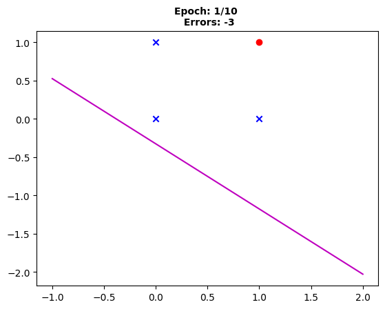 Fig. 1: “The decision boundary after the first epoch with three errors remaining to perfect classification.”
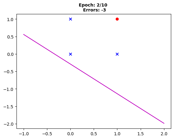 Fig. 2: “After the second epoch, the boundary has slightly shifted, yet three errors persist.”
 Fig. 3: “Post third epoch, the decision boundary’s evolution continues with still three misclassifications.”
 Fig. 4: “The decision boundary following the fourth epoch, three instances remain incorrectly classified.”
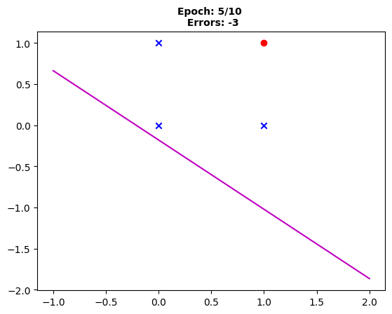 Fig. 5: “The fifth epoch shows maintained decision boundary movement, yet three errors remain.”
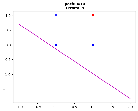 Fig. 6: “Post sixth epoch, slight changes are visible in the decision boundary, although three errors still persist.”
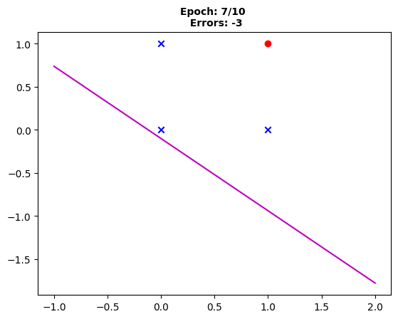 Fig. 7: “The decision boundary after the seventh epoch, with the same three instances misclassified.”
 Fig. 8: “The decision boundary evolution is steady after the eighth epoch, yet three instances remain incorrectly predicted.”
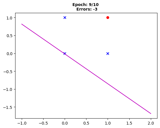 Fig. 9: “Following the ninth epoch, the boundary shifts but with the same count of three misclassifications.”
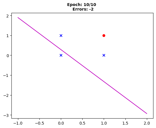 Fig. 10: “The conclusion of the tenth epoch shows the perceptron’s final decision boundary with only two errors, indicating improvement.”
The decision boundary’s movement as the weights and biases are updated portrays an essential aspect of the learning epochs. The decision boundary repositions itself to correctly distinguish the classes according to the perceptron updates, attempting to make the model’s predictions more accurate during the training process.
Through this visual representation, one can easily grasp the perceptron’s learning over iterations, making complex machine learning concepts more accessible and understandable.
Multilayer Perceptron
A multilayer perceptron (MLP) is a feedforward artificial neural network composed of one or more layers between the input and output layers. Additional hidden layers with nonlinear activation functions allow the network to learn nonlinear and more complex relationships between input and output patterns.
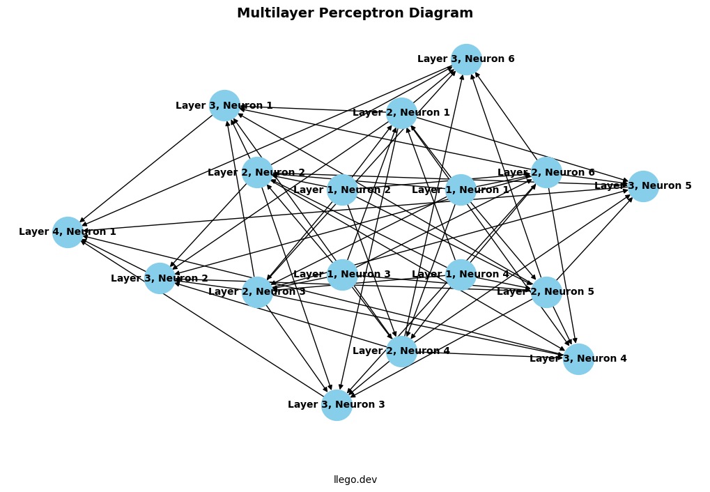 Fig. 11: “A multilayer perceptron diagram. See Python Code: Generating a Multilayer Perceptron Diagram section for the code to generate this diagram.”
Multilayer perceptrons commonly employ a variety of activation functions depending upon the complexity of the task and the nature of the input data. These include sigmoid, hyperbolic tangent (tanh), and rectified linear unit (ReLU) functions among others.
Training occurs through an iterative process called backpropagation, which relies on an algorithm called gradient descent to adjust the weights and minimize the loss function.
Gradient descent is an optimization algorithm that works by calculating the gradient (slope) of the loss function with respect to each weight parameter. The gradient indicates the direction and magnitude of change in the loss when a weight is varied. Using this gradient information, the weights are updated iteratively to move in the direction that reduces the loss. The size of each update step is controlled by the learning rate hyperparameter.
In backpropagation, the gradient is propagated backwards from the output layer through each hidden layer to efficiently calculate the influence of each weight on the overall loss function. The backpropagation algorithm enables training deep multilayer neural networks by overcoming the challenge of estimating the impact of each weight parameter in networks with multiple hidden layers.
By leveraging gradient descent within the backpropagation training process, the multilayer perceptron can learn complex functions and relationships between inputs and outputs. The addition of hidden layers and nonlinear activations empowers neural networks to model nonlinear decision boundaries and patterns that cannot be represented by simpler linear models like the perceptron.
Sigmoid Activation Function
The sigmoid activation function - that was prevalently used in earlier networks - maps input values into the range between 0 and 1, providing a smooth, normalized output:
def sigmoid(x):
    return 1 / (1 + np.exp(-x))
Hyperbolic Tangent Function
The hyperbolic tangent function, or tanh, is similar to the sigmoid but maps values into the range between -1 and 1. This leads to zero-centered output, which often helps the model to converge faster during the training phase:
def tanh(x):
    return np.tanh(x)
Rectified Linear Unit (ReLU)
Rectified Linear Unit, or ReLU, has become very popular in the last few years. It computes the function f(x)=max(0, x). In other words, the output is the input directly if it’s positive; otherwise, it’s zero. It has been found to speed up the training process significantly and is now widely used in the hidden layers of deep networks:
def relu(x):
    return np.maximum(0, x)
The output layer activation depends on the task - softmax for multiclass classification or sigmoid for binary classification.
Training occurs through an iterative process called backpropagation, which calculates the gradient of the loss function with respect to the weights in each layer. The weights are adjusted to minimize the loss using gradient descent or more advanced optimization algorithms like Adam or RMSprop:
Repeat until convergence:
    1. Forward propagation:
        - Input data propagates forward through network layers
        - Calculate outputs with activation functions
        - Generate loss at output layer

    2. Backward propagation:
        - Propagate loss backwards through network
        - Calculate gradient of loss with respect to weights

    3. Weight update:
        - Update network weights to minimize loss
        - Using gradient descent or advanced optimization algorithms
Multilayer Perceptron Implementation for Handwritten Digit Classification
In the example 3-layer MLP for classifying handwritten digits below, softmax activation has been used in the output layer. It’s important to note that this decision is an excellent practice when performing tasks that require multiclass classification. The reason for this is that the softmax function provides probabilities for each possible class which adds up to one, providing a clear winner and is thus suitable for these types of tasks.
import numpy as np
from scipy.special import logsumexp

# Define the size of the data.
sample_size = 500
input_size = 784 # 28x28 pixels
num_classes = 10
hidden_size = 32

# Initialize some random images and labels for the demonstration
X = np.random.rand(sample_size, input_size)
y = np.eye(num_classes)[np.random.choice(num_classes, sample_size)]  # One-hot encoded labels

# Model parameters
W1 = np.random.randn(input_size, hidden_size)
W2 = np.random.randn(hidden_size, num_classes)

# Bias vectors
b1 = np.zeros(hidden_size)
b2 = np.zeros(num_classes)

learning_rate = 0.001
epochs = 100

# Define cross-entropy loss
def cross_entropy(y_true, y_pred):
    return -np.sum(y_true * np.log(y_pred), axis=1).mean()

# Sigmoid activation
def sigmoid(x):
    return 1 / (1 + np.exp(-x))

# Softmax output activation
def softmax(x):
    e_x = np.exp(x - np.max(x, axis=-1, keepdims=True))
    return e_x / e_x.sum(axis=-1, keepdims=True)

# Training the model
for epoch in range(epochs):
    # Forward pass
    hidden = sigmoid(X @ W1 + b1)
    output = softmax(hidden @ W2 + b2)

    # Backpropagation
    dOutput = output - y
    dHidden = dOutput @ W2.T * hidden * (1 - hidden)

    # Calculate gradients and update weights
    grad_W2 = hidden.T @ dOutput
    grad_b2 = np.sum(dOutput, axis=0)
    grad_W1 = X.T @ dHidden
    grad_b1 = np.sum(dHidden, axis=0)

    W1 -= learning_rate * grad_W1
    b1 -= learning_rate * grad_b1
    W2 -= learning_rate * grad_W2
    b2 -= learning_rate * grad_b2

    # Print loss after each epoch
    if epoch % 10 == 0:
        loss = cross_entropy(y, output)
        print(f'Loss at epoch {epoch}: {loss}')
Sample output:
Loss at epoch 0: 7.311778885298072
Loss at epoch 10: 2.8659922350203204
Loss at epoch 20: 2.6192408762255237
Loss at epoch 30: 2.459668630422045
Loss at epoch 40: 2.3831059563985972
Loss at epoch 50: 2.3408736338089042
Loss at epoch 60: 2.3065959825847573
Loss at epoch 70: 2.277014330668523
Loss at epoch 80: 2.2509616685503806
Loss at epoch 90: 2.2273316668167547
Remember that this is a very basic neural network model. In practice, you would likely use a deep learning library like TensorFlow or PyTorch which will handle many details automatically and efficiently, like mini-batch processing, advanced optimizers, GPU acceleration, etc.
This demonstrates how a multilayer perceptron can learn complex functions and classify handwritten digits using backpropagation. The additional hidden layer enables modeling nonlinear decision boundaries that cannot be represented by a simple perceptron.
Modern deep neural networks extend this multilayer architecture with more layers and neurons for incredibly powerful feature learning. However, the multilayer perceptron marked a major advancement in neural network modeling capabilities.
Deep Learning and Various Neural Network Architectures
Deep learning, a subtype of machine learning, applies artificial neural networks modeled after the human brain to learn complex patterns from vast amounts of data. These networks are termed ‘deep’ due to containing many layers that progressively extract and transform features from raw input data.
A major innovation in deep learning is the Convolutional Neural Network (CNN). CNNs are specialized for processing data with a grid-like topology, like images, making them ideal for computer vision tasks. They utilize convolutional layers that apply filters to the input, reducing the dimensions while preserving important features. For example, the first layers may detect low-level features like edges, while deeper layers assemble these to detect higher-level features like faces.
CNNs were inspired by studies of the animal visual cortex by researchers like Hubel and Wiesel in the 1960s. But they only took off in the 2000s with advances in data, computation, and algorithms. CNNs now provide state-of-the-art accuracy for image and video analysis problems, like object classification and detection. Their introduction has been a crucial milestone in the progress of computer vision and deep learning as a whole.
Alongside CNNs, Recurrent Neural Networks (RNNs) and their advanced offshoots, Gated Recurrent Units (GRUs) and Long Short-Term Memory (LSTM) networks, have greatly contributed to the impact of deep learning. These networks are uniquely designed to handle sequential data by maintaining ‘memory’ of past inputs in the sequence. Therefore, they are particularly well-suited for problems involving time series data, such as financial forecasting, and text data, including language translation and sentiment analysis tasks.
The development and continuous enhancement of these various neural network architectures have ultimately extended the proficiency of deep learning operations in tackling a broader set of prediction problems.
Training Neural Networks
Training a neural network essentially involves optimizing the weights to minimize a loss function using some form of gradient descent or other optimization algorithms:
Loss Function
The loss function is used to measure how well the model’s outputs match the desired targets over the entire training dataset. Common loss functions include:
- Mean Squared Error (MSE) - Used for regression tasks to quantify the difference between predicted and actual values.
- Cross-Entropy Loss - Used for classification tasks to measure how close the predicted probabilities are to the true labels.
Optimization Algorithms
The gradient indicates how the loss changes as the weights are varied. Optimization algorithms make use of the gradient to update weights and minimize loss. Here are a few widely-used ones:
-
Gradient Descent: This algorithm iteratively adjusts the weights in a direction that reduces the loss. The size of the adjustment is controlled by the learning rate.
-
Momentum: This adaptation of gradient descent incorporates also a fraction of the update vector of past time steps to provide a bit of inertia and mitigate oscillations, which ultimately leads to faster convergence.
-
RMSprop (Root Mean Square Propagation): This technique introduces another modification to the gradient descent by normalizing the learning rate for each weight by considering its recent gradients, which often leads to faster and more effective convergence.
-
Adam (Adaptive Moment Estimation): Adam algorithm combines the methods from Momentum and RMSProp. It keeps an exponentially decaying average of past gradients (like momentum) and past squared gradients (like RMSProp). It’s well suited to problems that are large in terms of data and parameters, and has become one of the standard optimization methods in machine learning.
Hyperparameter Tuning
Important hyperparameters to tune neural network performance:
- Learning Rate - step size for optimization
- Batch Size - number of samples per gradient step
- Num Epochs - number of passes through training set
- Num Hidden Layers/Nodes - network architecture
- Activation Functions - sigmoid, tanh, ReLU etc.
Automated methods like grid search and random search can be used to find optimal hyperparameters.
Regularization
Techniques to reduce overfitting like L1/L2 regularization, dropout, data augmentation etc.
Challenges
Some of the challenges while training neural networks include:
- Non-convex Loss Function - many local minima: Neural networks’ loss function can have many local minimum points. This is a challenge as simple gradient descent methods might end up in poor local minima rather than the global optimum. To overcome getting stuck in poor local minima, techniques such as random initialization and adding noise to the gradients (both inputs to stochastic gradient descent) can help. The randomness introduced by these techniques helps expose the algorithm to more diversified areas of the loss function’s landscape, reducing the risk of converging into a suboptimal local minimum solution.
- Vanishing/Exploding Gradients - activations grow/shrink
- Overfitting - perform well on training but not test data
- Hyperparameter Tuning - many combinations to evaluate
- Computation Time - improved with GPUs and TPUs
Despite these challenges, ongoing research and improved algorithms continue to advance training effectiveness and efficiency. Proper training is key to enabling neural networks to generalize well and achieve optimal performance.
Evaluation Metrics
Once a neural network is trained, we need to gauge its performance. By using evaluation metrics, we can quantify the model’s predictive capabilities. For classification tasks, metrics such as accuracy, precision, recall, F1-score, and area under the ROC curve are commonly used. For regression tasks, mean squared error (MSE), root mean squared error (RMSE), mean absolute error (MAE), and R-Squared are usually employed.
Challenges and Limitations of Neural Networks
Despite their remarkable capabilities, neural networks are not without their limitations. For instance, they are infamous for being a “black box” because, while their predictions may be accurate, the logic behind these predictions is often uninterpretable and opaque. Moreover, training neural networks can be computationally costly and time-consuming, particularly with big data sets and complex architectures. They also require a significant amount of data to generalize effectively, which might not always be available. Furthermore, they are vulnerable to overfitting, especially when the network architecture is excessively complicated for the task at hand.
Applications of Neural Networks
Neural networks have broad applicability across many industries and use cases due to their flexibility to model diverse data patterns. Here are some common application areas and examples:
Computer Vision
Computer vision tasks like image classification, object detection, image segmentation and image generation have seen major advances thanks to convolutional neural networks (CNNs) like YOLO, R-CNN and generative adversarial networks (GANs). For instance, a CNN can be trained to identify objects in images or locate objects with bounding boxes accurately.
Natural Language Processing
Recurrent neural networks like long short-term memory (LSTM) networks excel at working with sequence data like text and speech. Applications include sentiment analysis to classify emotion in text, machine translation to convert between languages, and speech recognition to transcribe speech to text.
Recommendation Systems
Neural collaborative filtering models can uncover latent features in user-item interactions to power recommendation systems. For example, Netflix and Spotify use neural networks to predict user preferences and recommend movies, shows, songs and more.
Anomaly Detection
Autoencoder neural networks help profile normal vs. anomalous data patterns for applications like fraud detection and medical anomaly detection. They can identify abnormal customer transactions or detect abnormalities in medical tests.
Forecasting and Predictions
Recurrent neural networks perform well on temporal sequence forecasting tasks like sales, stock market or weather predictions. By analyzing historical patterns, they can forecast future trends.
These are just a few examples. Neural networks have broad applicability across many industries and use cases. The flexibility of neural networks to model diverse data patterns enables numerous real-world applications.
Real-World Applications: Industry Use Cases
Artificial Neural Networks are indispensable tools in various sectors, and their application is increasing as more industries recognize their immense potential. Let’s consider some specific examples:
Healthcare: Assisting doctors in diagnosis, neural networks are behind sophisticated image recognition systems like IBM Watson that can identify tumors and other abnormalities in medical images. Computational biology also uses neural networks to predict protein structures, a critical element in genetic research and drug discovery.
Finance: Neural networks help in predicting stock market trends, credit score modeling, detecting fraudulent transactions, and optimizing asset portfolio management. For instance, Mastercard’s Decision Intelligence is a good example of a neural network-based solution, aimed at reducing false declines and improving transaction approval rates.
Automotive: Autonomous driving is a pioneering field for neural networks. For example, Tesla’s Autopilot self-driving system primarily relies on neural networks to make sense of a diverse range of sensor inputs and decide on the most appropriate course of action (e.g., turning, accelerating, braking).
Technology: Apple’s FaceID technology on iPhones uses neural networks for facial recognition, demonstrating the role of these algorithms in secure biometric identification. Neural networks are also the backbone of recommendation algorithms used in streaming platforms like Netflix and Spotify, where they predict user preferences and recommend content accordingly.
E-commerce: Major e-commerce platforms like Amazon and Alibaba leverage neural networks for product recommendations, optimizing search rankings, and predicting customer purchasing behaviors. For instance, Alibaba’s intelligent recommendation system uses deep learning models and neural networks to predict what products will interest different customers based on their past behaviors.
Climatology: Neural networks play a crucial part in weather forecasting models, capable of learning patterns from historical climate data, and accurately predicting future weather conditions.
By shedding light on these use case scenarios across various sectors, we can fully appreciate the transformative potential of neural networks. The flexibility, robustness, and learning capability of these algorithms make them adaptable to different tasks, making them a cornerstone technology in current and future AI developments.
Key Takeaways
- Neural networks are inspired by biological brains and composed of artificial neurons
- The perceptron is a simple single layer neural network and one of the first learning algorithms
- Multilayer perceptrons can learn nonlinear functions using backpropagation
- Training involves optimizing weights to minimize a loss function
- Neural networks have applications in computer vision, NLP, recommendations, predictions, and more
- Ongoing research is advancing neural network capabilities and applications
In summary, the landscape of artificial intelligence and machine learning has been significantly altered by the advent of neural networks. Starting with simple models like the Perceptron, the evolution of this technology has led to complex deep learning architectures capable of impressive feats. Despite the challenges that come with training and implementing these models, their potential is undeniable. As further advancements are made and we continue to refine these algorithms, the future of neural networks appears promising, offering numerous exciting opportunities for scientific discovery and technological innovation.
Python Code: Generating a Multilayer Perceptron Diagram
import matplotlib.pyplot as plt
import networkx as nx

# Create a new directed graph using NetworkX
G = nx.DiGraph()

# Define the number of layers and the number of neurons in each layer
num_layers = 4  # Adjust this to the desired number of layers
neurons_per_layer = [4, 6, 6, 1]  # Adjust this list for the desired number of neurons in each layer

# Create nodes for each layer
for layer in range(num_layers):
    for neuron in range(neurons_per_layer[layer]):
        node_name = f'Layer {layer + 1}, Neuron {neuron + 1}'
        G.add_node(node_name)

# Add edges to connect the neurons in adjacent layers
for layer in range(num_layers - 1):
    for neuron1 in range(neurons_per_layer[layer]):
        for neuron2 in range(neurons_per_layer[layer + 1]):
            node1 = f'Layer {layer + 1}, Neuron {neuron1 + 1}'
            node2 = f'Layer {layer + 2}, Neuron {neuron2 + 1}'
            G.add_edge(node1, node2)

# Create a figure and plot the graph
plt.figure(figsize=(10, 6))

# Define the layout for the nodes
shell_layout_input = [[f'Layer {i + 1}, Neuron {j + 1}' for j in range(neurons_per_layer[i])] for i in range(num_layers)]

pos = nx.shell_layout(G, shell_layout_input)

nx.draw(G, pos, with_labels=True, node_size=1000, node_color='skyblue', font_size=10, font_color='black', font_weight='bold')

# Add labels
plt.title("Multilayer Perceptron Diagram", fontsize=14, fontweight='bold')

# Adding label to the plot
plt.text(0.5,-0.1,
         'llego.dev',
         size=10, ha='center',
         transform=plt.gca().transAxes)

# Show the plot
plt.axis('off')
plt.show()